
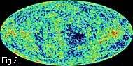
 The differential signal itself can be analyzed as well and examined for instance with regard to any non-random features of the fluctuations visible in the sky map. Fig.3 below shows a corresponding spectrum of the scales of the fluctuations in the map (angular power spectrum), apparently indicating a pronounced peak at 1o and a smaller peak at 0.3o (the theoretical curve (red) shows further peaks which do however not come out clearly in the data) (see http://map.gsfc.nasa.gov for more information).

A crucial element in the interpretation of the data is now the beam profile (window function) of the telescope, as it determines the angular resolution of the measurements. NASA quotes the resolution with 0.3o (average of V and W bands) which in itself should already raise some suspicion as this is rather close to the features visible in the data. The detailed profile of an individual beam for the individual channels is shown in Fig.4 below (taken from the paper by Page et al. (Fig. 2 there)).

This has been obtained by measuring the transit of a point source (Jupiter) through the beam (for the different channels) and essentially the same profile is also used for the difference signal (Eq.(11) in the paper, which is basically a simple average between the two beams correcting for slight differences between the two channels). However if two identical detectors measure a homogeneous background noise (which is the case for the CMB radiation), the difference between the count rates will not be zero but on average be equal to the square root of the count rates (the standard deviation). The beam profile for the differential signal is consequently not identical to the profile of the single beam but given by the square root of the latter (i.e. a function exp(-x2) would transform into exp(-0.5.x2) ) and the resolution correspondingly reduced. I have computed the associated error of the beam profile assuming Gaussian functions for the profiles with (e-fold) half-widths of 0.14o (W channels), 0.2o (V channel) and 0.3o (Q channel) (I estimated these values from Fig.4 above). This results in a profile for the individual telescopes A and B:
pA,B(θ)= [ 2*exp(-(θ/0.14)2) + exp(-(θ/0.2)2) + exp(-(θ/0.3)2) ]/4 .
where the W-Channel has been weighted double (as in the actual data analysis) because it contains twice the number of detectors.However, according to the above argument, for the differential signal of the two telescopes an additional factor 0.5 appears in the exponentials, i.e. the apparent profile is
pA-B(θ)= [ 2*exp(-0.5*(θ/0.14)2) + exp(-0.5*(θ/0.2)2) + exp(-0.5*(θ/0.3)2) ]/4 .
The error made by using pA,B(θ) instead of pA-B(θ) for the differential signal is consequentlyΔp(θ)= pA-B(θ) - pA,B(θ) .
I have plotted this function in Fig.5 below and it clearly exhibits a substantial peak concentrated near 0.2-0.3o (which corresponds to the location of the secondary peak in the data (Fig.3). The fact that the measured spectrum substantially decreases again before reaching 0.2o, whereas in the plot below it is still near the maximum at this point (note that the plot is in the opposite direction here), is likely to be due to circumstance that the above model formula for the beam profile is inaccurate near the center of the beam (i.e. the beam profile is actually flatter than assumed above). The apparent increase of the spectrum near 0.2o in the data is therefore most probably fictitious, which is also suggested by the rather large error bars in this range.
Whether the primary peak near 1o in Fig.3 is real or also a consequence of a systematic error in the data analysis requires further investigation. The only other experiment so far that unambiguously displays the main peak near 1o is ARCHEOPS and it is at least suspicious that the null-test for this experiment starts to fail exactly where the main peak develops (see Fig.6 below (top data points: Archeops Angular Power Spectrum; other points: null-tests) ). (the data for the BOOMERANG, MAXIMA and DASI experiments have too few data points and too large statistical errors to make any statements in this respect (see the corresponding data comparison)).

This suggests that the main peak is in fact also somehow caused by the details of the data analysis (subtractive data operations with almost-equal numbers only give correct results above a certain threshold of numerical accuracy and then become numerically unstable, which may be what has happened here (one should note the oscillatory and diverging behaviour of the Archeops null-test for decreasing angular scales)). It is therefore possible that the angular power spectrum (Fig.3), allegedly proving certain features of the Big-Bang Theory, is in fact an artifact of the data analysis but has nothing to do with the CMB at all (whatever the physical interpretation of the latter may be).
Update (April 2006)
With the Year 3- WMAP data having been released recently, my above analysis is in fact essentially confirmed: the difference between the 3- and 1-year maps shows residuals that have about the same amplitude as the second peak near 0.3 degree in the power spectrum. This is evident from Figs.3 and 9 in the Three Year Temperature Analysis which reveals a residual temperature fluctuation for the difference map of about ±20μK. Considering the circumstance that the difference map was smoothed with a 1 degree radius (which should have about halved the amplitude) this corresponds thus to the amplitude of the second peak (which is 50μK). The latter is therefore due to statistical fluctuations both in space and time which, as shown above, lead to an angular bias resulting in a residual signal at about 0.3o. It is by the way easy to show that the CMB fluctuation amplitude corresponding to the peak near 0.3 deg is what one would expect from a purely statistical fluctuation of the signal:if one considers the V-band (near 60 GHz) as representative for an average of the channels being taken into account for the power spectra, one arrives at the following figures: the energy flux of the cosmic microwave background near 60 GHz is 1.7.10-15 erg/cm2/sec/sr/Hz;
the surface of the telescope dish is about 1.8.104 cm2;
the effective integration time is 7.7.10-2 sec (see the WMAP-Radiometer Details );
the spatial angle of a beam with a half-width of 0.2 deg is about 4.10-5 sr;
the effective frequency bandwidth is 13 GHz (see the WMAP-Explanatory Supplement (PDF file, 2.1 MB)). Putting all these figures together, one finds that the telescope samples 1.7-15 .1.8.104 . 7.7.10-2 .4.10-5 .1.3.1010 = 1.2.10-6 erg within the data integration time. Now, since a photon at 60 GHz has an energy of 4.10-16 erg, this corresponds to 3.109 photons. The relative statistical error (standard deviation) associated with this is 1/√3.109 = 1.8.10-5 . For the difference of the two telescopes, the standard deviation would then be √2 times this value i.e. 2.5. 10-5, which is of the same order as the fluctuation observed at 0.3o (50 μK/2.7K = 1.9.10-5).